What a Network Engineer Needs to Know About ML Training

What one training step does

In the enterprise world, the network was a path. User to application. Application to database. Most of the time latency was not critical, because a human does not notice a millisecond.

Now the conversation is between GPUs inside one training job, and understanding what runs on top is no longer optional. A network engineer already does this for applications. You know which service talks to which, where the database sits, what DNS and the load balancers are doing.

An application has steps. A DNS call. An API call. A database call. A neural network has steps too, and the GPUs synchronize on every one.

This is my attempt to understand what a network engineer needs to know about a neural network in order to build the network that serves it. Two things come out of it. How many bytes cross your fabric, and how often. Both are decided before anyone asks you.

A neuron holds a number. Layers of them. Each number comes from the previous layer’s numbers: multiplied by weights, added to a bias, then passed through an activation function. The weights and the biases are the parameters. They are the knobs.

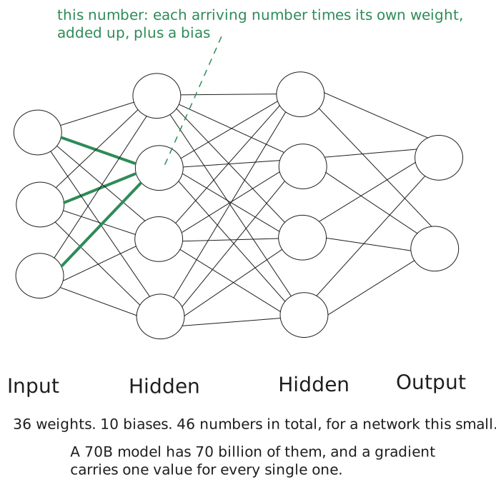
At the start every knob is random. The output is noise.

Training is turning the knobs until the output is right, and right has a definition here. The loss: one number that says how wrong this prediction was. Low loss, good model.

That is a search problem, and search problems are usually fine. This one is not, and the reason is the count.

A small model has a billion parameters. Turn one knob, run the model, see whether the loss moved. Do that a billion times and you have learned enough to take a single step. Then everything has changed and you start again.

You need something that tells you about every knob at once.

That is a gradient. It is the direction of steepest increase in the loss, and it has one component per parameter. Take its negative and you have the direction that lowers the loss. One calculation, every knob, and the size of each component tells you how much the loss cares about that particular weight.

Compute the gradient. Take a small step against it. Repeat. You are walking downhill on the loss, and the bottom is where the model is most accurate. That is gradient descent.

Computing that gradient still takes work, and backpropagation is what makes it affordable. One pass forward to get the prediction. One pass backward to get, for every weight and every bias in the model, how this training example wants it nudged.

One example, though.

Doing it exactly means running backpropagation over the entire training set and averaging the results. Slow enough that nobody does it. So the data is cut into mini-batches at random, and each step is computed on one mini-batch. It is an approximation, and it converges anyway.

Which makes the mini-batch the unit of everything that follows.

The five stages, in order:

Forward pass -> Loss -> Backpropagation -> Optimizer step -> Repeat

I am a network engineer, so I care about bytes.

FP32, BF16 and FP8 are floating-point formats. They trade precision and range for memory and speed.

FP32   32 bits   4 bytes
BF16   16 bits   2 bytes
FP8     8 bits   1 byte

There is one gradient value per parameter, so a gradient is the same size as the parameters. Call the parameter count N and the bytes per parameter B. N times B is how much data has to move. B is not a constant. Somebody chose it.

When the work is spread across GPUs in the simplest way, one mini-batch is one step. One step is one gradient sync. Batch size is picked for convergence and it arrives on your fabric as how often the cluster stops to agree.

Why one GPU is not enough

Ask how much memory a model needs, and most people multiply parameters by bytes. Seventy billion parameters in BF16 is 140 GB. That answer is correct for the weights of a model you are serving and wrong for training one, and the gap between those two numbers is the whole point.

During training, four things live in memory:

• the weights, 2 bytes. The working copy used for compute.
• the gradients, 2 bytes. One value per parameter, the same size as the parameters.
• the master weights, 4 bytes. An update is often smaller than the smallest change a 2-byte float can register, so adding it to the BF16 copy does nothing. The real weights are kept in FP32, and the BF16 copy used for compute is derived from them each step.
• the optimizer state, 8 bytes. Adam, the optimizer nearly everyone trains with, does not apply the gradient directly. It keeps two running numbers per parameter, a smoothed average of recent gradients and of their squares, and uses both to decide how far to move that parameter. Four bytes each.

Add them up: sixteen bytes per parameter, under one common mixed-precision Adam setup. Weights 2, gradients 2, master weights 4, momentum 4, variance 4.

Activations, the fifth thing. The forward pass produces intermediate values at every layer, and backpropagation needs them on the way back. Without activation checkpointing they are held for the duration of the step. They scale with batch size and sequence length rather than parameter count, so they are a separate term on top of the 16.

Seventy billion parameters times 16 bytes is 1,120 GB. Call it 1.1 terabytes.

An H100 SXM has 80 GB of GPU memory. It is a generation behind now, and it is still the part most clusters are built from and the one prices are quoted against. Fourteen provide exactly 1,120 GB in aggregate, before activations and other overhead. That is the arithmetic floor. A real build starts well above it.

Now the real question: memory or time.

Memory is what makes distribution mandatory. It is the reason the answer cannot be one GPU, no matter how patient you are.

But memory only gets you to fourteen. If memory were the whole problem you would buy two servers, wire them to one switch, and there would be no interesting networking here at all.

Time is what gets you to thousands. Training a 70B model on a few trillion tokens is somewhere around 10^23 to 10^24 floating-point operations. Even if it fit, one H100 at 40 percent utilization of its 989 TFLOPS of dense BF16 would take roughly eighty years. To finish in two weeks you need thousands of GPUs, and now they are in different racks, different rows, and the thing connecting them is a fabric somebody has to design.

Memory puts the model across GPUs. Time pushes those GPUs across racks. That is where the network becomes a fabric.

How training gets split

One GPU cannot hold the model, and one GPU cannot finish the work in time.

Adding GPUs is the answer to both. It does not tell you what each GPU should own.

A large model gives you three useful places to cut: the batch, the math inside each layer, or the layers themselves.

Each cut makes a different kind of traffic.

Data parallelism: cut the batch

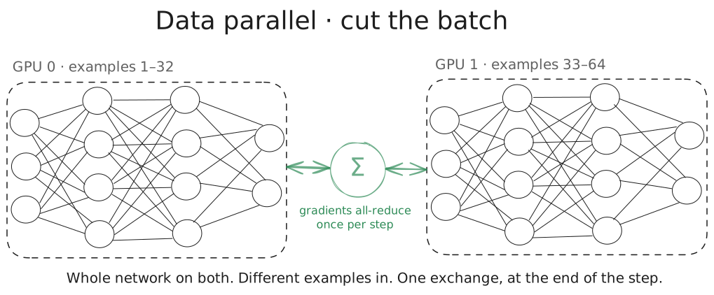
Start with the simplest one.

Every GPU holds a full copy of the model. The batch gets divided, and each GPU works on different examples.

At the end of the step, every GPU has its own opinion about how the weights should move. Those opinions have to be combined before the model can take the next step. That is the all-reduce, one communication operation involving a whole group of GPUs.

What crosses the wire is the gradient. One value per parameter.

For a 70-billion-parameter model communicating gradients in BF16, the raw gradient tensor is 140 GB. Implementations divide it into buckets and begin reducing them while backpropagation is still running, but the total still follows the parameter count.

The problem is memory.

Pure data parallelism copies the entire training state onto every GPU. At sixteen bytes per parameter, that is 1.1 TB for a 70B model. Copying it onto eight GPUs does not make it smaller.

FSDP and ZeRO fix this by removing the copies. At full sharding, the parameters, gradients, and optimizer state are divided across the data-parallel group.

But a GPU still needs a layer’s weights before it can compute that layer. So it gathers them from the other GPUs on the way forward, then reduce-scatters the gradients on the way back.

The memory problem did not disappear. It arrived on the network.

Full sharding spends bandwidth to buy HBM.

Tensor parallelism: cut the operation

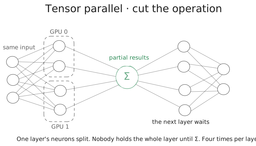
Sometimes the model cannot fit even after the training state is sharded. The next cut goes inside the layer itself.

Take one matrix multiplication and split its weight matrix across several GPUs. Each GPU calculates part of the answer for the same input.

A partial answer is useless by itself. The GPUs have to combine their results before the layer can continue.

This is the chatty one.

In the original Megatron tensor-parallel layout, each transformer layer requires two collectives during the forward pass and two during the backward pass. An 80-layer model produces 320 collectives per step.

The exact collective changes with the implementation. The network consequence does not. Communication happens inside the layer, and the next calculation waits for it.

Each exchange is smaller than the full gradient because it carries activation-sized data. But it happens hundreds of times, directly in the critical path.

Pipeline parallelism: cut the layers

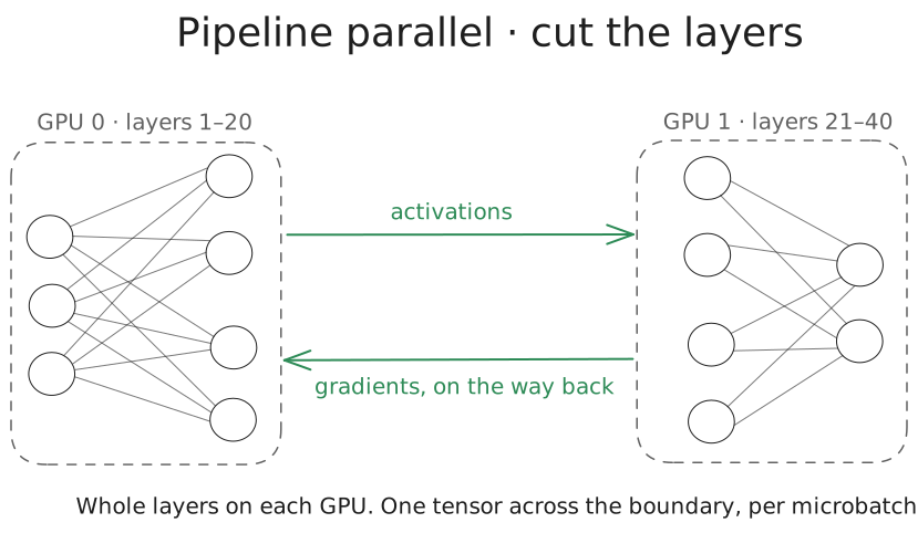
GPU 0 gets layers 1 to 20. GPU 1 gets layers 21 to 40. The activation crosses the boundary going forward, and its gradient comes back during backpropagation.

The problem is the bubble. While the first GPU works, the later stages wait. So the batch is split further, into microbatches, and several chunks move through the pipeline at once to keep the stages busy.

That makes it point-to-point traffic between adjacent stages, one boundary tensor per microbatch.

The topology follows the cut

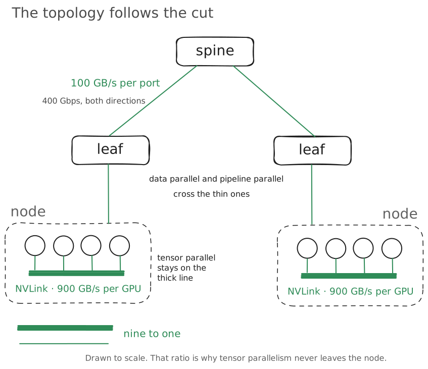
Tensor parallelism needs the fastest and shortest connection available. Its hundreds of blocking exchanges belong inside the NVLink domain (a group of GPUs connected through NVIDIA’s scale-up interconnect).

An H100 SXM provides 900 GB/s of aggregate bidirectional NVLink bandwidth per GPU. A full-duplex 400 Gbps network port provides 100 GB/s in aggregate.

Nine to one.

I have spent fifteen years deciding which traffic is allowed to cross which boundary. Here the first boundary is drawn by arithmetic.

Tensor parallelism stays inside the NVLink domain. Put hundreds of blocking collectives on the slower scale-out fabric and the step time follows them.

Data parallelism can travel farther. Gradients for the later layers are ready before backpropagation finishes, so part of the communication can overlap with compute. That makes it the natural traffic to carry across NVLink domains and onto the scale-out fabric.

Full sharding makes that pattern busier because the parameter gathers cross the same boundaries.

Pipeline parallelism sits between them. It sends activation tensors between adjacent stages instead of running a collective across the whole group. That traffic crosses NVLink domains more easily than tensor-parallel traffic.

Large training jobs often combine all three. Tensor parallelism cuts the work inside an NVLink domain. Pipeline parallelism connects several of those domains. Data parallelism spreads the remaining replicas across the fabric.

The placement is deliberate. Get it wrong and expensive GPUs spend their time waiting for a cheaper link.

The number people get wrong

Under mixed-precision Adam, sixteen bytes per parameter live in HBM, the GPU’s local high-bandwidth memory.

That does not mean sixteen bytes per parameter cross the fabric. You would never size a link off the size of the LSDB. A router holds far more state than it ever puts on the wire, and nobody has ever confused the two. This is that mistake, in a place where nobody has learned to spot it yet.

A BF16 gradient contains two bytes per parameter. For a 70B model, that is a raw gradient payload of 140 GB. It matches the 140 GB weight figure for the same reason: both are the parameter count times two bytes. The collective algorithm and group size then determine how much traffic each physical link carries.

Storage precision and communication precision are separate decisions.

Use the HBM number to size the fabric and you overstate the raw gradient payload by eight times.

Why GPUs have to synchronize

All three cuts create the same problem. One GPU’s result is not enough to continue.

Data parallelism shows it most clearly.

Every GPU starts the step with the same model, but works on a different slice of the batch. During backpropagation, each GPU calculates gradients from the examples it saw.

At the end of the step, GPU 0 has one set of gradients. GPU 1 has another. Neither is wrong. Neither represents the full batch.

Imagine one weight in the model. The examples on GPU 0 say that weight should move up. The examples on GPU 1 say it should move down. Each GPU has an opinion based on part of the evidence.

If they apply those gradients independently, the model copies stop being copies. GPU 0 updates its weights one way. GPU 1 updates them another way. The next step begins with two different models.

Data parallelism has turned into separate training runs.

The gradients have to be combined into one batch-wide result. Every GPU must receive that same result and apply the same weight update. Only then do all replicas begin the next step with identical weights.

That is what the all-reduce does. Every GPU contributes its values, they are summed, and every GPU gets the total back. Divide that total by the number of participants and you have the batch-wide average.

The location of the dependency changes with the type of parallelism.

With tensor parallelism, each GPU holds part of a layer’s result. The next operation cannot begin until those partials are combined.

With pipeline parallelism, one stage produces the activation the next stage needs. During backpropagation, the dependency runs in the other direction.

Sometimes the wait happens once per optimizer step. Sometimes it happens hundreds of times inside the model. The reason is the same.

Splitting the work splits the answer. Synchronization puts it back together.

In every network I have built, a slow participant hurts itself. A page loads late. A replica falls behind and catches up. Here the slow one holds everyone else at its own speed.

The barrier belongs to the algorithm. No fabric design can remove it. Every GPU has to wait because the next calculation depends on the combined result.

And the traffic arrives together. This is not many flows coinciding by chance. It is one event, by construction, thousands of times an hour.

The fabric decides how long that wait lasts.

A neural network has steps too, and the GPUs synchronize on every one.